From attenuation measurements to a reconstructed image

What the detectors actually see

You open a CT series and see a clean axial slice of a chest: lung, ribs, and soft tissue. To understand how that displayed image was formed, follow it backward to what the gantry records.

A CT gantry rotates an x-ray source around the patient. Opposite the source is a detector array. For each source position, the detectors record how much x-ray intensity reaches them after travelling along many paths through the body. The result is a collection of one-dimensional attenuation profiles from different directions, called projections. A detector reading integrates what happened along a path; it does not identify the attenuation at one particular point inside the patient. A single projection therefore cannot, by itself, distinguish air from bone at a location along that path.

In a simplified line-integral model, if I₀ is the incident intensity and I is the transmitted intensity, the logarithmic quantity -ln(I/I₀) is related to the line integral of the attenuation coefficient. This conversion gives the reconstruction process a more useful representation of the measurements, but it does not turn one detector reading into a slice. The projections are commonly arranged by angle and detector position as a sinogram.

X-ray source
    |
    | beam through patient
    v
Detector row: transmitted intensity along many paths
    |
    | logarithmic conversion gives one projection
    | repeat and stack over many angles
    v
Sinogram
    |
    | reconstruction algorithm
    v
Axial slice: computed pixels

The slice you read is the output of the final reconstruction step. The detectors produced the projection data at the beginning of the chain.

Reconstruction makes the image

To get from projections to a two-dimensional image, the scanner runs a reconstruction algorithm. The classical method is filtered back-projection (FBP): projection values are distributed back across the image plane, the contributions from many directions are combined, and a filter controls the frequency response of the result. Iterative and model-based methods instead update a candidate image while comparing its predicted measurements with the recorded projections under a model of noise and image formation. The details differ, but both approaches produce an image by computation.

When raw projection data are retained and the system permits re-reconstruction, the same measured data can be processed with different settings. A useful mental model is Iθ = R(P; θ): P denotes the projection data, R the reconstruction process, and θ the chosen settings. Holding P fixed does not imply that Iθ is fixed. Changing θ can change the spatial resolution, noise, and appearance of the resulting image.

The settings represented by θ can include the reconstruction kernel, slice thickness, field of view, matrix size, and reconstruction algorithm. Two images formed from the same projection data can therefore be different images and can produce different quantitative measurements. This is why reconstruction belongs in the provenance of a measurement rather than in a footnote.

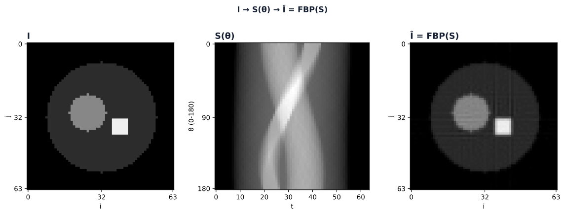
Simplified 2D parallel-beam model: 60 noiseless projections, no dose, helical motion, or ring/cone artefacts; one simplified FBP implementation whose result depends on the filter, interpolation and discretisation. The reconstructed image is an algorithm’s output under stated settings — no pixel in it is a direct detector reading or a direct measurement of tissue.

Quantitative, but not context-free

CT is quantitative in an important but conditional sense. Reconstructed values are often expressed on the Hounsfield scale, where water is defined as 0 HU and air is conventionally near -1000 HU. This scale makes it possible to use attenuation values as part of a measurement, but it does not make every value unambiguous or independent of the imaging protocol.

A voxel value is the output of a reconstruction applied to measured projections. The kernel, slice thickness, noise level, energy spectrum, contrast phase, and partial-volume effects can all affect what that value represents in a particular image. Approximate tissue ranges are useful orientation, not universal diagnostic thresholds. CT is quantitative under a stated protocol; it is not a direct measurement of one infinitesimal point in the body.

Because reconstruction changes image texture and resolution, it can be a consequential source of variation in quantitative imaging, especially for measurements that respond to spatial frequency and noise. Its relative importance depends on the feature, protocol, and other processing choices; this chapter does not rank it against every other source of variation. The practical consequence is narrower and more useful: record the reconstruction whenever reporting a measurement.

The next section turns that rule into a case. A public paired CT collection makes it possible to separate what changes when the patient is scanned again from what changes when one acquisition is reconstructed in more than one way.