Case study: RIDER robustness

The previous section separated repeatability, reconstruction agreement, and reproducibility as different measurement questions. The public RIDER Lung CT Version 3 dataset makes the distinction concrete because it contains both a same-day repeat and multiple reconstructions of each scan. The original design paper by Zhao et al. documents the paired same-day/repositioning context; its repeatability analysis used one thin-section reconstruction for tumour-size measurements, whereas the six-reconstruction package belongs to the current TCIA v3 record. It is a useful illustrative case, but it remains bounded: it characterises specified measurement behavior under one dataset and one declared analysis contract. It does not establish biomarker validity, clinical utility, or reproducibility across every scanner, site, or protocol.

A paired design with two comparison families

RIDER contains lung-cancer patients scanned again on the same scanner on the same day, with matched tumour segmentations and multiple reconstruction settings for each scan. The short interval supports a repeatability question: the biological target is expected to have changed little, while repositioning, respiration, physiology, acquisition noise, segmentation, and extraction can still differ. The reconstruction settings support a separate question: what happens when the same acquisition is represented with a different reconstruction?

The design can be pictured as a grid. Each patient has two scan rows and reconstruction settings arranged across the columns. Comparing the two scans within one column forms the test-retest family. Comparing columns within one row forms the reconstruction-agreement family.

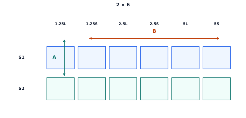
Schematic design, not a specific patient dataset: the grid shows structure, not values. The six settings do not exhaust reconstruction space, and each family is analysed separately on real data using an appropriate agreement statistic.

The same patient and the same reconstruction column are essential for the first comparison. The question is whether the feature agrees across the near-identical repeat, not whether two arbitrary scans have similar distributions. The same acquisition basis and one scan row are essential for the second comparison. The question is whether changing the reconstruction changes the feature, not whether a different patient or a different clinical population has a different value.

Neither family answers the broader reproducibility question by itself. The test-retest comparison does not test different scanners or sites. The reconstruction comparison deliberately varies a reconstruction axis rather than the full acquisition environment. They must therefore be analysed separately, even though they can be represented in one design matrix.

What is held fixed, and what is varied

A meaningful comparison begins with a declared measurement contract. The feature choice, image type, region and label, geometry, resampling and interpolation, intensity handling, discretisation, dimensionality, neighbourhood, and matrix aggregation must be fixed or explicitly assigned to the axis being studied. The purpose is not to pretend that all other sources of variation disappear, but to make the intended comparison identifiable.

For test-retest repeatability, the patient, scanner, session context, and reconstruction setting define the comparison basis. A same-day repeat can still change the patient’s position and the measured image. If the segmentation is redrawn independently, segmentation variation is included as part of the tested chain. The resulting agreement describes repeatability of that complete chain under the declared conditions.

For reconstruction agreement, the acquisition is the comparison basis and the reconstruction setting is the deliberate variation. A different reconstruction can change voxel values and spatial appearance. Depending on how the regions are produced and represented, it can also be accompanied by differences in geometry or segmentation. Those effects are not reasons to relabel the comparison as a generic reproducibility study. They are part of the question that must be recorded: how much does the downstream measurement change when this reconstruction axis changes?

A result from either family is conditional on the choices that define it. A feature calculated after a different discretisation, mask, or resampling operation is not a clean replicate of the original feature unless that change is part of the planned comparison. The agreement statistic cannot repair an unrecorded change in the contract.

A one-parameter sensitivity experiment

The paired design can be combined with a small sensitivity experiment before any aggregate interpretation is attempted. Begin with visual and geometric sanity checks. Confirm that the image and tumour mask occupy the intended spatial relationship, that the region is not empty or obviously misplaced, and that the relevant image and label geometry have been interpreted consistently. A precise feature value from a misplaced region is still a precise answer to the wrong input.

Next, choose one feature and write down the fixed extraction contract. For example, a single GLCM summary such as JointEntropy can be calculated from one declared image, one declared mask, one geometry and interpolation path, one intensity-handling rule, one discretisation rule, and one dimensionality and aggregation convention. These choices remain fixed while one parameter is perturbed. The exact values are part of the case record; no particular parameter value is a universal recommendation.

The prediction should be made before the second extraction. If the selected change in binWidth separates several intensity values that were previously assigned to one grey level, it is reasonable in that particular region to expect the GLCM probability mass to be redistributed and the Joint Entropy to change. A prediction that the value will increase may be appropriate for a specific observed grey-level pattern, but it is not a rule that smaller bins always raise entropy or move every texture feature in the same direction.

Run the original and perturbed calculations with the remaining contract held fixed, then compare the values and the discretised representations. If the result matches the local prediction, the experiment makes the grey-level alphabet’s role visible. If it does not, explain the mismatch mechanistically rather than calling the extractor unreliable by default. A nearly uniform region, a small number of voxels, values near bin boundaries, intensity clipping, or an interaction with the chosen matrix and aggregation can all change the expected direction. The mismatch is evidence about this defined sensitivity experiment, not evidence of a change in the tumour.

The same design can vary one geometric or interpolation choice instead, but that is a different perturbation. Changing bin width and resampling together would make the result harder to attribute. The one-parameter rule is therefore an experimental control: vary one declared cause, observe the feature, and describe what the comparison actually tested.

The test-retest analysis

For the repeatability analysis, extract the same feature from the two same-day scans of each patient using the same declared contract and the same reconstruction column. Preserve the pairing. A feature that changes between the paired scans has shown sensitivity under the full repeatability chain, but the pair alone does not say whether repositioning, physiology, segmentation, noise, or another step contributed most.

Across patients, agreement can be summarised with an appropriate ICC or CCC and accompanied by paired differences, uncertainty, and plots that show the identity relationship. The coefficient is a descriptive result for the tested cohort and conditions. It is not a property of the feature name independent of the measurement process, and it is not an absolute error in the feature’s units.

The reconstruction analysis uses a different pairing. Within one scan row, compare values obtained from different reconstruction settings according to a declared comparison scheme. The acquisition is treated as fixed for the purpose of the experiment, while the reconstruction varies. A feature may agree across the sampled settings, disagree across them, or behave differently at different settings. Each outcome describes the tested reconstruction robustness; none establishes behavior at unsampled settings or across different sites.

The two analyses should not be pooled into one coefficient. A same-day test-retest difference and a same-acquisition reconstruction difference arise from different perturbations and carry different interpretation. Combining them would make a single number look more general while concealing which question it answered.

The anti-tuning rule

Do not choose binWidth, spacing, interpolation, or another extraction parameter because it produces the most favorable downstream score. That would turn a measurement-sensitivity study into outcome-informed feature selection. The purpose of this case is to observe what a declared contract does, not to search for a contract that wins.

If a later analysis asks whether one parameter choice improves prediction, that is a new prespecified modelling question. Reporting guidance such as the CLEAR radiomics reporting checklist and TRIPOD+AI places parameter selection, feature selection, and other data-dependent steps within the declared model-development/evaluation design; these are reporting frameworks, not empirical validation. Fit those choices using only the permitted training portion and apply them to held-out data. The resulting predictive analysis must therefore be evaluated within the appropriate validation design. The RIDER robustness case stops earlier. It describes how the measurement behaves under repeatability, reconstruction, and controlled perturbation comparisons.

The strongest conclusion available here is correspondingly narrow. The case can show that a feature is sensitive or comparatively stable under a specified condition, and it can help identify which additional contrast would localise a possible source of variation. It cannot show that the feature measures the intended biology, improves prediction, or benefits a clinical decision. Those claims require separate evidence.

Having separated the paired comparison families and protected the experiment from parameter tuning, the chapter can now ask what happens after measurement performance has been characterised. The next section, Harmonisation and the model handoff, examines how multi-site differences, robustness decisions, and downstream modelling should be connected without treating harmonisation as a substitute for understanding the original measurement.

Sources

• Ye S, Lim JY, Huang W. Statistical considerations for repeatability and reproducibility of quantitative imaging biomarkers. BJR Open. 2022;4(1):20210083. doi:10.1259/bjro.20210083, PMID 36452056.
• Lin LI. A concordance correlation coefficient to evaluate reproducibility. Biometrics. 1989;45(1):255-268. doi:10.2307/2532051, PMID 2720055.
• Pfaehler E, et al. Phys Imaging Radiat Oncol. 2021;20:69-75. doi:10.1016/j.phro.2021.10.007, PMID 34816024.
• Haarburger C, et al. Scientific Reports. 2020;10:12688. doi:10.1038/s41598-020-69534-6.
• Zhao B, Schwartz LH, Kris MG, Riely GJ. Coffee-break lung CT collection with scan images reconstructed at multiple imaging parameters (Version 3) [Dataset]. The Cancer Imaging Archive. doi:10.7937/K9/TCIA.2015.U1X8A5NR, collection page.
• Zhao B, et al. Radiology. 2009;252(1):263-272. doi:10.1148/radiol.2522081593, PMID 19561260, PMCID PMC2797680.
• Kocak B, et al. CLEAR radiomics reporting checklist. Insights into Imaging. 2023;14:75. doi:10.1186/s13244-023-01415-8.
• Collins GS, Moons KGM, Dhiman P, et al. TRIPOD+AI statement. BMJ. 2024;385:e078378. doi:10.1136/bmj-2023-078378.