Discretisation changes the measurement

The preceding section built a GLCM from a small image whose voxels had already been assigned grey levels. That construction exposes a problem that is easy to miss in a software pipeline: the matrix does not see the original intensity scale directly. It sees the grey-level alphabet created by discretisation.

Changing the bin width can therefore change the matrix even when the image, mask, and anatomy remain identical. The resulting feature values are not measurements of biological change. They are values of a defined feature under different discretisation rules. Treating them as interchangeable hides a change in the measurement contract.

The grey-level alphabet is part of the feature

In the fixed-bin-width convention documented by PyRadiomics, the intensity axis is divided into equally wide bins. The unshifted bin index is

bin_index = floor(HU / binWidth)

The implementation then shifts the labels so that the smallest grey level inside the region becomes 1. The complete mapping is

X_b = floor(HU / binWidth) - floor(min(HU_ROI) / binWidth) + 1

The shift changes the labels used in the matrix, but not which voxels share a bin. The bin width determines which intensity differences remain distinct and which are collapsed into one grey-level category.

This is an implementation-specific convention, not a universal definition of discretisation. The IBSI fixed-bin-size method uses floor((X - X_min) / w) + 1, with the bins anchored to the minimum intensity in the region. Here, the ROI minimum is the anchor for this worked example; a general IBSI contract may instead declare a lower-bound, including a re-segmentation lower bound. PyRadiomics instead uses the zero-anchored floor(X / w) and then applies the constant relabelling shown above. The two rules can therefore assign boundary values to different categories. Their shared consequence is that discretisation is feature-determining: it affects the grey-level alphabet, which affects the matrix, which affects the feature. The PyRadiomics customization documentation and the IBSI reference paper describe the respective workflows.

The bin width used below is an illustrative choice, not a recommendation or a claim about a universal software default. The point is to follow the same values through two different definitions.

A five-value demonstration

Consider five intensity values inside one small region:

HU values:  [ -987,  -982,  -978,   -50,   -30 ]

Apply the unshifted floor operation for two bin widths:

HU	binWidth = 5	binWidth = 25
-987	floor(-987/5) = -198	floor(-987/25) = -40
-982	floor(-982/5) = -197	floor(-982/25) = -40
-978	floor(-978/5) = -196	floor(-978/25) = -40
-50	floor(-50/5) = -10	floor(-50/25) = -2
-30	floor(-30/5) = -6	floor(-30/25) = -2

At binWidth = 5, the first three values occupy three different grey-level categories. At binWidth = 25, they all occupy the same category. The two soft-tissue values also share a category at the larger width. After the implementation’s constant relabelling, the category labels may be different, but the grouping of values remains the same.

If these values have fixed spatial positions, the smaller bin width preserves distinctions that the larger width removes. A GLCM built from the two discretised versions can therefore contain different grey levels, different occupied cells, and different probabilities. The same reasoning applies to run-length, size-zone, dependence, and neighbourhood-difference matrices. The anatomy did not change; the representation supplied to the matrix did.

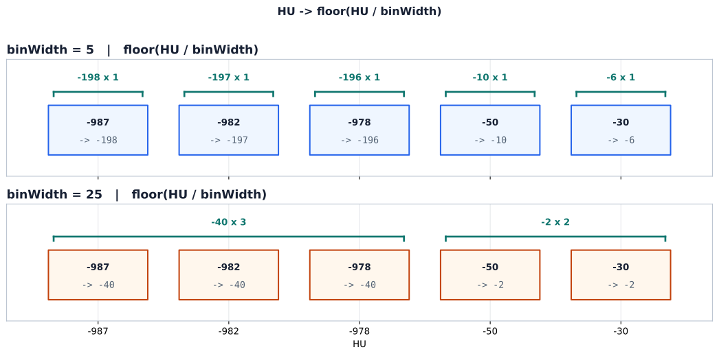
The inputs stay fixed while binWidth changes the grey-level alphabet; neither setting is intrinsically superior.

What the example does and does not predict

The five-value construction supports a specific prediction: for these values, binWidth = 5 preserves three distinctions in the first group, whereas binWidth = 25 collapses them. That is an auditable change in the input to the matrix.

It does not support a universal rule that smaller bins always produce a higher entropy, a higher contrast, or a particular movement in every texture feature. Those directions depend on the intensity distribution, the spatial arrangement, the matrix family, the feature formula, and any direction or aggregation convention. Finer bins can expose more grey-level states, but they can also change how probability is distributed among matrix cells in ways that do not produce a monotonic change in every summary. Coarser bins can remove distinctions without making every feature move in the same direction.

Entropy and contrast make the distinction clear. Entropy responds to how widely probability mass is spread across matrix states. Contrast weights transitions according to their distance from the diagonal. A change in bin width can alter both summaries, but neither one can be inferred from the bin width alone. The two settings in the demonstration are not intrinsically superior; they define different resolutions of the intensity relationships. Which resolution is appropriate depends on the intended measurement and the study design.

Reporting the complete contract

A texture value without its discretisation rule is incomplete. Reporting JointEntropy = 2.3 without saying how the grey levels were assigned leaves the matrix that produced the value unspecified. A reproducible report must place the binning rule alongside the other choices that determine the measurement: the image type, region and label, physical grid, resampling and interpolation, intensity transformations or clipping, dimensionality, neighbourhood, distance, direction, symmetry treatment, aggregation, and implementation semantics.

This does not mean that every analysis must use identical choices. It means that a reader must be able to tell whether two values are the same operational quantity or values produced under different contracts. A change in bin width can be a deliberate sensitivity analysis when the rest of the pipeline is held fixed. It must not be mistaken for a change in the measured object.

The same discipline applies when a feature is later used in a predictive analysis. Choosing the bin width after inspecting which setting gives the best downstream score turns a measurement-definition choice into outcome-informed feature selection and therefore model development. Reporting guidance such as the CLEAR radiomics reporting checklist and TRIPOD+AI treats such data-dependent choices as part of the declared development/evaluation design; these are reporting frameworks, not empirical validation of a model. The resulting score no longer evaluates a prespecified measurement process. The bin width and the rest of the extraction contract should be fixed before the relevant result is used, or the choice must be treated as a model-development step and evaluated within the appropriate validation boundary.

Discretisation therefore links the three levels of the construction. The grey-level alphabet determines what distinctions the image representation retains. That alphabet determines the spatial matrix. The matrix determines the numerical summary called a texture feature. If any one of those levels changes, the resulting value may be a different measurement even when the underlying anatomy is unchanged.

Once the discretisation rule and the rest of the contract are fixed, a further question becomes possible: does the feature remain sufficiently stable when the conditions that should leave the target unchanged are repeated or perturbed? The next section, Can this feature be trusted?, examines repeatability, reconstruction agreement, reproducibility, and the evidence needed to characterise measurement performance.

Sources

• Zwanenburg A, Vallières M, Abdalah MA, et al. The Image Biomarker Standardisation Initiative: standardized quantitative radiomics for high-throughput image-based phenotyping. Radiology. 2020;295(2):328-338. doi:10.1148/radiol.2020191145, PMID 32154773, and published full text at PMC7193906.
• PyRadiomics documentation - radiomic feature definitions and customizing the extraction.
• Kocak B, et al. CLEAR radiomics reporting checklist. Insights into Imaging. 2023;14:75. doi:10.1186/s13244-023-01415-8.
• Collins GS, Moons KGM, Dhiman P, et al. TRIPOD+AI statement. BMJ. 2024;385:e078378. doi:10.1136/bmj-2023-078378.