How a voxel gets an (x,y,z) position

So the array has no location. How does a voxel acquire one? This section builds the affine map from integer voxel index (i, j, k) to physical patient coordinate (x, y, z) — an affine relation, not a purely linear one: a linear direction-and-spacing term plus the origin translation — and works it through real numbers. Once you can write the affine, slice ordering, resampling and CT↔SEG comparison all become arithmetic.

Where is voxel (0,0,0)?

The patient-coordinate position of a voxel is determined by the three geometry quantities already met: origin, spacing, and direction. The first voxel (0,0,0) sits at the origin. To reach any other voxel you step along the three axes, each step scaled by that axis’s spacing and pointed along that axis’s direction. String those steps together and you have the affine.

The geometry, in DICOM’s words

This is the durable reference for pixel index ↔ patient coordinate mapping. It follows the DICOM Image Plane Module (PS3.3 C.7.6.2.1.1).

DICOM pixel indices use (i, j) with:

• i = column index (0 … Columns−1): increasing i traverses a row of the transmitted image matrix — a matrix/display traversal convention, not an anatomical left or right direction.
• j = row index (0 … Rows−1): increasing j traverses a column of the transmitted matrix — likewise a traversal convention, not an anatomical top/bottom direction.

Which anatomical way each index points is decided by ImageOrientationPatient, not by the words “row” and “column”.

ImageOrientationPatient (0020,0037) = six direction cosines:

• first triplet [rx, ry, rz] = the row direction = direction of increasing i;
• second triplet [cx, cy, cz] = the column direction = direction of increasing j.

PixelSpacing (0028,0030) = [row spacing, column spacing]:

• first value = row spacing = distance between adjacent rows = step when row index j increases by 1;
• second value = column spacing = distance between adjacent columns = step when column index i increases by 1.

The cross-coupling is the trap (the next section is devoted to it): the row direction cosine pairs with the column spacing, and vice versa.

The in-plane equation

For a single frame, the patient coordinate of the pixel at (i, j) is:

P(i, j) = P0
        + i · (column spacing) · [rx, ry, rz]      # move along a row (i increases)
        + j · (row spacing)    · [cx, cy, cz]      # move along a column (j increases)

where P0 = ImagePositionPatient (0020,0032) of the first (top-left) pixel of this frame. The slice normal adds the third axis — that is the business of the slice-order section.

A worked numeric example

Take a simple axis-aligned axial slice (the common case), so the row points along +x and the column along +y:

ImageOrientationPatient = [1, 0, 0,  0, 1, 0]      # row=+x, col=+y
PixelSpacing            = [0.8, 0.8]               # [row spacing, col spacing] mm
ImagePositionPatient    = [-200, -150, 42.0]       # P0, LPS mm

Where is the pixel at column i = 100, row j = 200?

P(100, 200) = [-200, -150, 42.0]
            + 100 · 0.8 · [1, 0, 0]     =  [+80,    0,   0]
            + 200 · 0.8 · [0, 1, 0]     =  [   0, +160,  0]
            -------------------------------
            = [-120, +10, 42.0]  mm (LPS)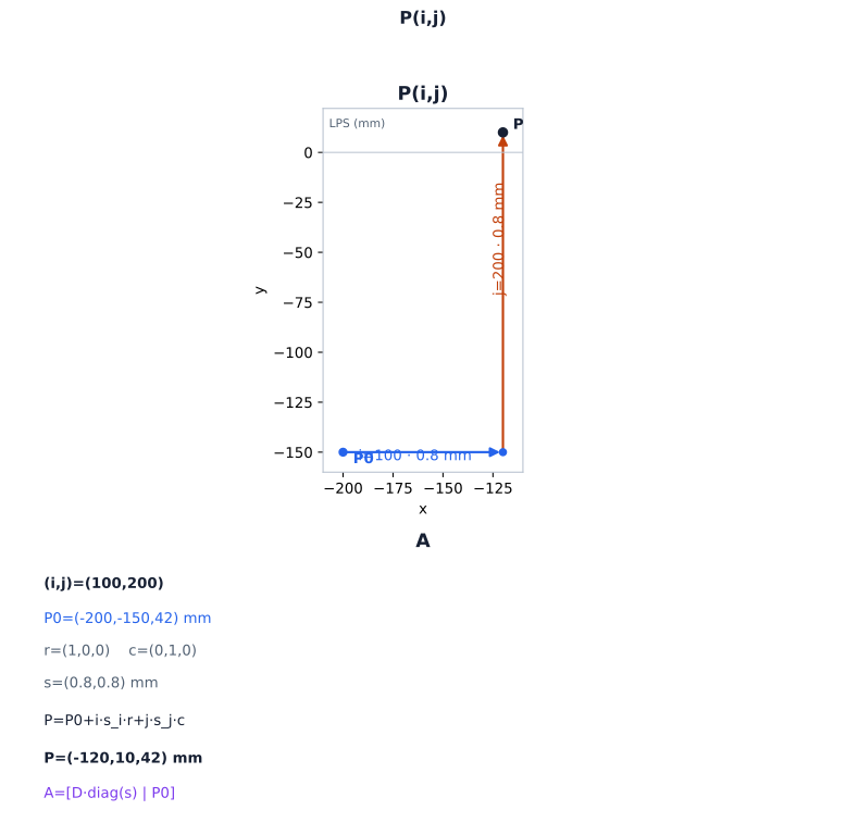

The plotted point is this section’s worked example: from P0, each step of i moves 0.8 mm along the row direction and each step of j moves 0.8 mm along the column direction, and (i, j) = (100, 200) lands at (−120, +10, 42.0) mm in LPS.

Notice the z-component is unchanged (42.0) — but scope that to this example. It holds because the slice is axis-aligned axial: both in-plane direction cosines have zero z components. In an oblique, coronal, or sagittal plane the in-plane direction vectors carry z components, so moving within one slice can change patient z — moving between slices is not the only way z changes. In this worked example the third image axis is supplied by the inter-slice geometry — the slice normal (the slice-order section).

Read the result as: “voxel index (100, 200) on this slice is the physical point 120 mm to the right of and 10 mm posterior of the origin, at height 42 mm.” The array index became a millimetre position in the patient. That conversion is the affine doing its one job. Every “is this mask in the right place?” question reduces to applying this map and comparing coordinates.

Two checks inside the example are worth making explicit. The origin voxel (i = 0, j = 0) is just P0 = [-200, -150, 42.0] — the origin is literally the position of the first pixel. And increasing i by 1 adds 1 · (column spacing) · row direction = 1 · 0.8 · [1,0,0] = [0.8, 0, 0], i.e. 0.8 mm along +x. That 0.8 mm is the column spacing. So “spacing” is not an abstract metadata field — in this worked example, it is the centre-to-centre sample step along the relevant image axis. Spacing determines that coordinate step, but it is not automatically the voxel’s tissue support, slice thickness, sensitivity kernel, or spatial resolution. The arithmetic derived a coordinate step from the geometry, not a universal physical size for one voxel.

The affine as a matrix

Pack origin, spacing and direction into one 4×4 matrix A (homogeneous coordinates) and the map becomes a single multiply:

[ x ]     [   D·diag(s)   |  origin ]   [ i ]
[ y ]  =  [               |         ] · [ j ]
[ z ]     [               |         ]   [ k ]
[ 1 ]     [   0   0   0   |    1    ]   [ 1 ]

where D is the 3×3 direction-cosine matrix (columns = axis directions), diag(s) is the 3×3 diagonal matrix that scales each axis by its spacing, and origin is the three-component translation column. In ordinary three-dimensional form the relation is affine — linear direction and spacing plus a translation — and only this homogeneous 4×4 representation folds the translation into a single matrix multiply. This is exactly what TRACE-CT’s build_affine() constructs from IOP/IPP/spacing, and what SimpleITK carries internally as GetOrigin()/GetSpacing()/GetDirection().

What can go wrong even with the right affine

• Oblique volumes. If the gantry was tilted, the direction matrix is not identity and the axes are not aligned with +x/+y/+z. Apply the full matrix; do not assume “axial means identity”.
• Per-slice origin changes. Each slice has its own ImagePositionPatient. The in-plane affine is shared across a regular series, but P0 differs per slice — that is precisely the information the slice-order section uses to order slices.
• LPS vs RAS. For ordinary human (BIPED) imaging, DICOM and ITK/SimpleITK keep physical coordinates in LPS, while 3D Slicer stores its internal coordinates in RAS; the boundary conversion negates the x and y components. Omitting that conversion — or applying it twice — can reflect or misplace coordinates. It is a risk to check for, not a guaranteed visible mirror: readers and writers may perform the conversion automatically.

With the affine in hand, the remaining hazard is not the transform itself but the conventions feeding it — which index is which, and which spacing pairs with which direction. The next section takes up that row/column trap in full: how NumPy and SimpleITK index the same voxel in opposite orders.

Sources

• DICOM PS3.3, Image Plane Module (C.7.6.2) and Image Position and Image Orientation (C.7.6.2.1.1, Equation C.7.6.2.1-1) — pixel index semantics, ImageOrientationPatient, PixelSpacing, ImagePositionPatient, and the pixel-to-patient-coordinate mapping. (current edition)
• SimpleITK, fundamental concepts — origin, spacing, direction, and the index-to-physical-point mapping (GetOrigin()/GetSpacing()/GetDirection()), including the NumPy↔SimpleITK array conversion and its opposite dimension order. (docs)
• 3D Slicer documentation, coordinate systems — Slicer’s internal RAS convention, the LPS↔RAS boundary conversion, and the affine image transform. (docs)
• TRACE-CT, scripts/seg_decode_resample.py, build_affine() — bounded project implementation evidence for constructing the affine from IOP/IPP/spacing. (commit 7aaf308c)