Texture matrices from first principles

The previous section treated texture as one of five ways to summarize spatial relationships in the measurement table. That description is useful only if the counting operation is visible. A name such as GLCM can otherwise sound like a property that the image possesses naturally. It is not. A texture feature is calculated by first assigning image values to a finite set of grey levels, counting a specified relationship among those levels, and then summarizing the resulting matrix.

Why texture needs a grey-level alphabet

A CT image is represented by intensity values on a numerical scale, but a texture matrix does not usually count every possible intensity as a separate category. Suppose one tried to count how often one raw intensity occurred next to another in a region of interest. The possible pair states would be numerous, and most would occur rarely or not at all. The resulting matrix would be large and sparse, making it a poor representation of the spatial patterns the calculation is intended to summarize.

Discretisation replaces the continuous or finely sampled intensity axis with a declared grey-level alphabet. Voxels whose values fall in the same interval receive the same grey level. Texture is then calculated from the relationships among those assigned levels, not directly from the raw intensity labels. The choice of intervals is therefore part of the measurement definition. It decides which differences remain visible to the matrix and which differences are deliberately treated as equivalent.

Discretisation is part of the definition

In the fixed-bin-width convention documented by PyRadiomics, the intensity axis is divided into bins of equal width, with the bins spaced from zero. The unshifted bin index is

bin_index = floor(HU / binWidth)

The implementation then shifts the labels so that the smallest grey level inside the region becomes 1. Written together, the mapping is

X_b = floor(HU / binWidth) - floor(min(HU_ROI) / binWidth) + 1

The shift changes the labels but not which voxels share a bin. For understanding the construction, the important operation is the division by the chosen binWidth and the flooring of the result.

For example, using an illustrative binWidth = 25 and showing the unshifted floor values:

HU	floor(HU / 25)
-40	-2
-30	-2
-20	-1
+30	+1

The values -40 and -30 therefore enter the same grey-level category, while -20 and +30 enter different categories. The subsequent shift gives the categories implementation-friendly labels; it does not restore the intensity distinctions that the bin width removed.

This is a PyRadiomics convention, not a universal synonym for IBSI discretisation. The IBSI fixed-bin-size method uses floor((X - X_min) / w) + 1, with the bins anchored to the minimum intensity in the region. PyRadiomics instead uses the zero-anchored floor(X / w) and then applies the constant relabelling shown above. The difference matters because the two rules can assign boundary values to different grey-level categories. The shared methodological consequence is that discretisation is feature-determining: changing the rule can change the matrix and therefore the texture value. The PyRadiomics customization documentation and the IBSI reference paper describe the respective conventions.

A directional GLCM built by hand

Take a small region that has already been discretised to the grey levels {1, 2, 3}:

1 1 2 3
1 2 2 3
2 2 3 3
1 2 3 3

A GLCM, or grey-level co-occurrence matrix, counts how often a grey level i occurs beside a grey level j under a specified spatial relationship. Choose the relationship “one voxel to the right”: a horizontal neighbour at distance 1. Walking from left to right in each row produces these ordered pairs:

Row	pairs
row 1	(1,1) (1,2) (2,3)
row 2	(1,2) (2,2) (2,3)
row 3	(2,2) (2,3) (3,3)
row 4	(1,2) (2,3) (3,3)

There are twelve pairs because each of the four rows contributes three horizontal neighbours. Put the first member of each pair on the matrix rows and the second member on the matrix columns:

        j=1   j=2   j=3
i=1  [   1     3     0  ]
i=2  [   0     2     4  ]
i=3  [   0     0     2  ]

The entry in row i and column j is the number of times the ordered transition i -> j occurred for this offset. Dividing every entry by the total of 12 converts the counts into probabilities. Matrix features are then calculated from that probability representation.

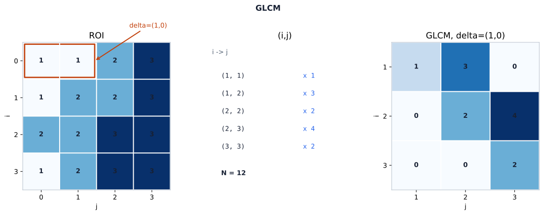
This teaching matrix counts only the directed left-to-right offset: each ordered pair contributes once, giving N=12. IBSI GLCM construction and default PyRadiomics combine opposite offsets into a symmetric matrix; the displayed asymmetric tally is the contribution from delta=(1,0) before symmetrisation, not the standard or default final GLCM.

This small example makes the direction a visible part of the result. If the opposite offset were counted, the ordered pairs would be reversed. If several directions were included, several matrices would exist. A calculation could keep them separate, combine them before calculating a feature, or calculate a feature for each and aggregate the resulting values. Those choices are not interchangeable for nonlinear summaries:

feature(average_i(matrix_i)) is not generally identical to average_i(feature(matrix_i))

Consequently, “GLCM” does not fully specify a measurement. The offset, distance, direction, symmetry convention, and aggregation rule must also be known.

Two summaries of one matrix

The count matrix is not a picture of biology. It is a compressed description of the transitions produced by one discretised image and one neighbourhood rule. Different mathematical summaries of the same matrix can emphasize different properties.

Joint Entropy describes how broadly the probability mass is distributed across the occupied matrix cells. If most of the mass is concentrated in a few states, entropy is lower; if the mass is spread across more states, entropy is higher. In the worked matrix, five cells are occupied and the mass is distributed among them, so the entropy is moderate. Entropy does not, by itself, weight a cell according to its distance from the diagonal. A transition from level 1 to level 3 and a transition from level 1 to level 2 occupy different cells, but their distance from the diagonal is not what the entropy summary directly measures.

Contrast does use distance from the diagonal. Its pair contribution is weighted by (i - j)^2, so transitions between levels that are far apart contribute more strongly than transitions between equal or neighbouring levels. In the worked matrix, the occupied off-diagonal cells are only one grey-level step from the diagonal. Moving comparable probability mass to cells such as (1,3) or (3,1) would increase Contrast because those cells have a larger squared distance from the diagonal.

The two summaries are therefore complementary rather than interchangeable. A smooth progression through nearby levels can have low contrast while still spreading probability across several matrix cells and producing moderate entropy. A feature name such as Joint Entropy or Contrast identifies a mathematical summary of a constructed matrix; it does not establish that the summary measures a particular tissue mechanism.

The other texture families follow the same general pattern with different counting objects. GLRLM counts runs of equal grey levels along a direction. GLSZM counts connected equal-level zones. GLDM counts neighbourhood dependencies under a declared distance and dependence rule. NGTDM compares a voxel’s grey level with the local neighbourhood average. Each matrix requires its own spatial definition before its features can be interpreted.

Direction, dimensionality, and aggregation

The worked matrix is planar and uses one directed horizontal offset. A two-dimensional analysis may build matrices within each slice and then aggregate them. A three-dimensional analysis can include relationships across adjacent slices in the volume. These are different constructions even when they use the same mask and the same intensity values. A 2D GLCM and a 3D GLCM of one region are therefore different quantities, not two displays of one underlying number.

The physical grid matters as well. A neighbour in an array is interpreted through the image geometry and resampling contract. Slice spacing, anisotropy, and the chosen target grid affect which physical relationships are represented by a nominal offset. The same nominal distance can describe a different physical separation in two images if their geometry differs.

Aggregation introduces another layer of meaning. Combining directional or distance-specific matrices before calculating a feature gives the feature one joint probability structure. Calculating separate feature values and averaging them gives each matrix a separate summary before combination. Neither can be assumed to be the universal interpretation of the family name. A reproducible report must state the dimensionality, offsets or distances, directions, symmetry treatment, and aggregation convention.

Consequences for the measurement table

The worked construction also shows why a texture column cannot be compared by name alone. Two values called JointEntropy may have been calculated from different grey-level mappings, different physical grids, different neighbourhoods, or different aggregation rules. They can be scientifically useful for their respective questions, but they are not automatically the same measurement.

Discretisation, direction, dimensionality, and aggregation are not cosmetic settings applied after texture has been measured. They determine the matrix from which the feature is calculated. A change in bin width can merge or separate grey levels. A change in direction can replace one set of ordered transitions with another. A change from planar to volumetric construction can add through-plane relationships. A change in aggregation can alter the probability structure before the nonlinear summary is evaluated.

This is also why texture features should be treated as related candidates, not as independent biological observations. Several features may summarize different aspects of the same matrix, and matrices built from related directions, distances, or filtered images may reuse much of the same information, which can induce dependence or correlation without guaranteeing it for every pair. The next analysis step must preserve the distinction between a mathematical summary, the measurement contract that produced it, and any later biological or predictive interpretation.

The next section examines that contract under a controlled change: Why binWidth changes the answer follows the same voxels through different discretisation choices and shows how changing the grey-level alphabet changes the resulting texture measurement.

Sources

• Zwanenburg A, Vallières M, Abdalah MA, et al. The Image Biomarker Standardisation Initiative: standardized quantitative radiomics for high-throughput image-based phenotyping. Radiology. 2020;295(2):328-338. doi:10.1148/radiol.2020191145, PMID 32154773, and published full text at PMC7193906.
• PyRadiomics documentation - radiomic feature definitions and customizing the extraction.