Longitudinal change and absolute measurement error

Suppose a synthetic example gives a feature value of 2.41 before treatment and 2.68 afterwards. It is tempting to write that heterogeneity increased. The two numbers do not establish that conclusion. Their difference is another image-derived measurement, and it can reflect biology, acquisition, segmentation, geometry, preprocessing, or implementation. Before interpreting it, define what change means and establish how much movement the measurement produces when the target is intended to be unchanged.

Change is a derived measurement

For baseline value f1 and follow-up value f2, an analysis might define change as an absolute difference f2 - f1, a relative change (f2 - f1) / f1, or a log-ratio log(f2) - log(f1). These are not interchangeable. They have different units and different behaviour near zero, and a log-ratio is not suitable for a feature that crosses zero or whose sign has no meaningful interpretation. The choice belongs in the frozen methods rather than being selected for the clearest figure.

The interval between scans and the treatment or other context between them are also part of the definition. A six-week interval and a six-month interval mix treatment effect, natural evolution, and background physiology differently. A delta without its interval and context is incomplete, just as a temperature without units is incomplete.

Repeatability and detectable change

Test-retest and perturbation studies estimate how much a feature moves when the intended biological target should be nearly unchanged. CCC is a dimensionless relative agreement or reliability quantity whose value depends on between-subject spread. It can describe relative concordance, but it does not supply an absolute error in the feature’s units. For longitudinal detectability, select and justify one absolute error quantity compatible with the feature’s scale, estimand, error structure, repeatability or reproducibility conditions, protocol, and intended decision. A report need not use all of the available quantities.

Within-subject SD or SEM estimates within-subject measurement error on the measurement scale under declared repeatability conditions; wCV is appropriate only when a multiplicative or ratio-scale error model is justified. Under the usual independent, approximately normal repeatability-error model, a repeatability coefficient can be written as RC = 1.96 * sqrt(2) * within-subject SD, or as RC = 2.77 * wCV on an appropriate relative scale. Bland-Altman limits of agreement (LoA), mean paired difference +/- 1.96 * SD of differences, describe bias and dispersion for a defined pair of methods or conditions; their assumptions, heteroscedasticity, and estimation precision must be assessed. A smallest detectable change (SDC) is an individual-level convention often written as 1.96 * sqrt(2) * SEM. It is algebraically related to RC under matching assumptions, but its terminology and estimand are not universally interchangeable with LoA or with a QIBA profile claim. Choose one compatible absolute error model, state its assumptions, and justify it for the intended decision rather than presenting all four quantities as jointly required.

Compare an observed change with the prespecified criterion or interval produced by that model. A change inside the criterion is not distinguishable at the chosen measurement resolution under its assumptions; crossing it makes the change a candidate for investigation, not proof of biological response. Scanner, protocol, contour, and region changes can also create a large difference. There is no universal percentage at which a delta becomes real, and no absolute threshold can be derived from CCC alone.

A schematic thought experiment

Consider two synthetic features. Entropy moves from 3.10 to 3.14 while a schematic same-day repeatability band has half-width 0.05. Contrast moves from 40 to 52 while a schematic same-day swing is approximately 25 percent. The first change sits inside its illustrative band. The second is only slightly beyond the interval from 30 to 50 implied by the illustrative swing. Neither change, by itself, licenses a biological interpretation. Reversing the entropy example to 3.10 to 3.35 would create a candidate worth investigating, not a proven treatment effect.

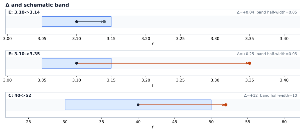
Schematic values, not clinical measurements. Each displayed band half-width is an arbitrary illustrative input, not an estimated SD, SEM, RC, LoA, SDC, or clinical threshold. A real decision band requires a prespecified, justified error quantity from repeatability characterization of the stated feature, pipeline, cohort, and conditions. Crossing it creates a candidate for investigation, not proof of biology; remaining inside does not prove absence of response. The figure establishes no universal percentage threshold.

What changes between timepoints

The measurement layer is now a two-timepoint problem. The scanner, reconstruction, contrast timing, slice thickness, and protocol may differ. The lesion must be segmented at both timepoints under a documented procedure. Its size and tissue composition may change, so a feature can partly reflect that the two regions now contain different mixtures of tissue. Registration matters for voxelwise comparisons, whereas a feature-table delta can be defined without pretending that corresponding voxels are aligned. Resampling, clipping, discretisation, and implementation semantics must be held comparable or deliberately modelled. A peritumoral region adds changes in surrounding anatomy such as oedema or atelectasis to the list.

These moving parts make pairing essential. Analyse within-patient change or use a model that represents the repeated-measures structure. Split, resample, and fit any data-dependent transformation at the patient level. Putting one patient’s baseline in training and follow-up in testing leaks subject information even if the two rows have different timestamps. A change score does not erase the dependence created by its two source measurements.

What published delta studies can and cannot show

Published pancreatic-cancer studies provide useful examples of the design rather than a universal performance guarantee. One analysis nested in a prospective trial used paired pre-treatment and post-treatment CT, protocol-consistency exclusions, inter-observer filtering, percentage deltas, and internal, non-fully-nested bootstrap validation; its reported predictors included volume change alongside texture changes. A separate study used discovery and external cohorts and reported independent external evaluation for OS and DFS. Its margin model used validation data during the mCOM procedure, so it should not be described as a clean independent external margin evaluation. It combined clinical and delta-radiomic information rather than treating radiomics as a replacement for clinical variables. These are study-specific analyses whose cohorts, endpoints, splits, and results require direct source inspection before their numerical claims are generalized.

The methodological lesson is narrower and more durable. A delta model should, when relevant to the estimand, be compared with prespecified clinical and volume-change baselines on the same patient-level splits. It should disclose the delta definition, timing window, segmentation procedure, protocol exclusions, and stability characterization. A review can reasonably place this evidence tier below a mature, externally tested measurement standard while protocols and validation remain heterogeneous; that qualification is not a reason to discard longitudinal measurement, but a reason to limit the claim.

The chapter has moved from a number, through its measurement system and region, to agreement, uncertainty, and change. Chapter 6 now returns to the contents of the measurement table: feature families, texture matrices, and discretisation. It can ask which radiomic features are useful only because this chapter has made clear what it means for one to be measured and compared.

Sources

• De Robertis R, et al. CT texture analysis and delta radiomics in predicting R0 resection after preoperative chemotherapy in resectable pancreatic ductal adenocarcinoma. Translational Oncology. 2026. doi:10.1016/j.tranon.2026.102900.
• Wang K, et al. Delta radiomic features predict resection margin status and overall survival in neoadjuvant-treated pancreatic cancer patients. Annals of Surgical Oncology. 2024;31:2608-2620. doi:10.1245/s10434-023-14805-5, PMID 38151623.
• Duan et al. CT quantitative imaging after neoadjuvant therapy in pancreatic ductal adenocarcinoma. Gland Surgery. 2026;15:201. doi:10.21037/gs-2026-0239, PMID 42591759.
• Quantitative Imaging Biomarkers Alliance (QIBA), RSNA — official QIBA information.
• QIBA. CT Tumor Volume Change for Advanced Disease, Clinically Feasible Profile. doi:10.1148/qiba/20220721.
• Ye S, Lim JY, Huang W. Statistical considerations for repeatability and reproducibility of quantitative imaging biomarkers. BJR Open. 2022;4(1):20210083. doi:10.1259/bjro.20210083, PMID 36452056.
• Bland JM, Altman DG. Statistical methods for assessing agreement between two methods of clinical measurement. Lancet. 1986;1(8476):307-310. doi:10.1016/S0140-6736(86)90837-8, PMID 2868172.
• de Vet HCW, Terwee CB, Knol DL, Bouter LM. When to use agreement versus reliability measures. Journal of Clinical Epidemiology. 2006;59(10):1033-1039. doi:10.1016/j.jclinepi.2005.10.015, PMID 16980142.
• Collins GS, Moons KGM, Dhiman P, et al. TRIPOD+AI statement. BMJ. 2024;385:e078378. doi:10.1136/bmj-2023-078378.
• Bernett J, et al. Guiding questions to avoid data leakage in biological machine learning applications. Nature Methods. 2024;21:1444-1453. doi:10.1038/s41592-024-02362-y.