Timing, weighting, and sequence contrast

Readout timing is the contrast choice

After excitation, T1 recovery and T2 decay proceed together. The sequence cannot make those tissue properties disappear; it can choose when and how to sample the evolving signal. In a conventional spin-echo mental model, two timing parameters make that choice legible.

Repetition time (TR) is the interval between successive excitations of the same nominal location. A shorter TR leaves less time for longitudinal magnetisation to recover before the next excitation, so differences in T1 have more influence on the signal. A longer TR reduces that dependence. Echo time (TE) is the interval from excitation to the echo that is sampled. A longer TE allows more transverse decay before readout, so differences in T2 have more influence. A shorter TE reduces that loss.

This is why a short-TR, short-TE acquisition is commonly described as T1-weighted, while a long-TR, long-TE acquisition is commonly described as T2-weighted. A long TR combined with a short TE tends to reduce both T1 and T2 effects and is often called proton- density-weighted. These are weighting regimes, not direct measurements: the labels say which tissue differences dominate the displayed contrast under that sequence, not that a single image reports a tissue’s T1 or T2 value.

The useful equation is a deliberately limited mental model. With proton-density effects and other sequence details held simple, a spin-echo-like signal can be written as S ≈ ρ(1 − e^(−TR/T1))e^(−TE/T2). Changing TR changes the recovery term; changing TE changes the decay term. Real sequences add flip-angle effects, refocusing or gradient timing, echo trains, inversion preparation, flow, susceptibility, and reconstruction choices. The formula explains the direction of the timing effect; it is not a universal forward model for every clinical image.

Reading relative brightness

Brightness is always a relationship within the displayed image. In a common clinical orientation, fluid is often dark relative to other tissues on T1-weighted images and bright on T2-weighted images, while fat is often relatively bright on T1-weighted images. Those tendencies are useful for identifying the contrast family, but they are not guarantees: anatomy, pathology, sequence implementation, field strength, suppression, flow, and display settings all matter.

Weighting	Typical timing tendency	Relative appearance used for orientation	Common interpretive use
T1-weighted	short TR, short TE	fat often bright; fluid often dark	anatomy and appropriate post-contrast assessment
T2-weighted	long TR, long TE	fluid often bright; muscle often relatively dark	fluid-sensitive assessment
PD-weighted	long TR, short TE	proton-density differences are emphasised while T1/T2 effects are reduced	anatomy where proton-density contrast is useful

The table compresses the preceding explanation rather than replacing it. For example, CSF that is bright in a fluid-sensitive brain acquisition suggests T2-dominant contrast, but it does not reveal the numerical T2 of the CSF. A quantitative T2 estimate requires an acquisition with suitable variation in echo times and a model or fitting procedure.

The same caution applies to gadolinium. A gadolinium-based contrast agent can shorten T1; when it reaches a tissue, its presence may therefore increase signal on an appropriate T1-weighted acquisition. The observed enhancement depends on the sequence, timing, agent distribution, and tissue context. It is a comparison between examinations or regions under stated conditions, not a property that was already measured by the pre-contrast image.

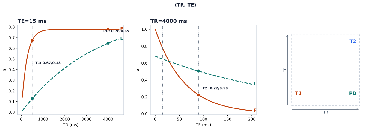
Two tissue models and one closed-form equation — no grey-scale display, scanner calibration, proton-density differences, or multi-compartment behaviour. A single conventional T1- or T2-weighted image does not provide quantitative T1 or T2 values; mapping signal to those parameters requires an appropriate quantitative protocol and model fitting.

Sequence families are implementation families

The timing model also explains why sequence names should not be treated as interchangeable image labels. A sequence family specifies a way of preparing, refocusing, encoding, and sampling the magnetisation; its actual contrast is still determined by parameters and implementation.

Family	Operational idea	Consequence for the image
Spin echo (SE)	excitation followed by a refocusing pulse and an echo	a useful reference model for T1/T2 contrast
Turbo/fast spin echo (TSE/FSE)	several refocusing echoes are collected after an excitation	faster coverage with contrast also affected by the echo train
Gradient echo (GRE)	gradients form the echo without a conventional 180° refocusing pulse	fast acquisitions with greater sensitivity to T2* effects in many implementations
Inversion recovery (IR)	an inversion pulse precedes excitation and is timed with TI	a selected tissue can be suppressed
STIR	an IR preparation chosen for a short-TI fat null	fat-suppressed contrast, with its own timing and tissue dependencies

The last two families extend the same idea rather than contradicting it: timing is an instrument for selecting contrast. Inversion recovery and signal suppression makes that instrument concrete by following the longitudinal magnetisation through its zero crossing.

Sources

• Abi Berger, “Magnetic resonance imaging” — pulse sequences and the relationship between tissue relaxation and MR contrast.
• Stanford Medicine Body MRI Research Group, MRI Physics Education Materials — public visual orientation on contrast mechanisms and pulse sequences.
• Ridgway JP. Cardiovascular magnetic resonance physics for clinicians: part I. J Cardiovasc Magn Reson. 2010;12:71. doi:10.1186/1532-429X-12-71. (Full text)
• Stanford Center for Cognitive and Neurobiological Imaging. MR Signal Equations. Permanent revision oldid=2295. (Technical reference)
• Smith TE, Steven A, Bagert BA. Gadolinium Deposition in Neurology Clinical Practice. Ochsner J. 2019;19:17-25. doi:10.31486/toj.18.0111. (Full text)