Case study: one acquisition, several reconstructions

A patient may be scanned once while the archive contains several image series: a thin 1.25 mm lung-kernel stack, a thick 5.0 mm soft-tissue stack, a coronal reformat, and a scout. These are not interchangeable duplicates. The first two can be separate reconstructions of acquired data; a reformat is a derived view of an image volume, and a scout is a different acquisition product. Their shared examination does not make their pixels equivalent.

The reconstruction setting is part of the image

The slice is the output of a reconstruction algorithm. Projection data cannot be assumed to remain available after the patient leaves the gantry, but when they are retained and the scanner or a workstation permits re-reconstruction, the same acquired data can be processed with different settings. Each resulting image is archived as its own series or representation.

One important setting is the reconstruction kernel: a frequency-selective choice that trades spatial resolution against noise and edge sharpness. A sharp lung- or bone-oriented setting can preserve more high-frequency detail while making noise and fine edges more prominent. A smoother soft-tissue setting can reduce visible noise while changing the spatial detail that remains prominent. The names are vendor- and protocol-dependent; labels such as B70f, B30f, and B40f in an example should not be treated as universal categories.

When a DICOM object records this choice, the attribute identified as ConvolutionKernel (0018,1210) is a useful place to look for provenance. Its normative semantics remain a source-review question rather than something to infer from a filename.

This is why a texture measurement from a sharp-kernel image can differ from the same measurement on a smoother image formed from the same acquired data. The kernel is not a descriptive afterthought: it is one of the variables that may determine the image supplied to the measurement step.

The RIDER six-setting matrix

A bounded public example is the TCIA RIDER Lung CT v3 collection (collection page, DOI 10.7937/K9/TCIA.2015.U1X8A5NR, CC BY 4.0). The collection description used for this case describes 32 people with non-small-cell lung cancer, two scans on the same day, and six reconstruction settings for each scan. That design makes the case useful because it places a near-repeat comparison beside a comparison of reconstruction settings. It is a dated illustrative dataset example, not a claim that every CT examination contains these six outputs.

The six settings are three slice thicknesses crossed with two kernel families:

              lung kernel (L)      standard kernel (S)
 1.25 mm      1.25L                1.25S
 2.5  mm      2.5L                 2.5S
 5    mm      5L                   5S

Read a label as thickness plus kernel family: 1.25L is a 1.25 mm image with the lung-style setting, while 5S is a 5 mm image with the smoother standard setting. In this illustrative matrix, L and S are labels for the two families, not a promise that every scanner uses the same names or the same filter implementation.

Two different comparisons live inside this matrix. Keeping them separate is the methodological decision that makes the case useful:

Comparison in the case	Intended contrast	Question
Scan 1 1.25L vs Scan 2 1.25L	same person and reconstruction, with the scans acquired close together under the study design	test–retest repeatability: how much the measurement varies under near-identical conditions
Scan 1 1.25L vs Scan 1 5S and the other within-scan setting pairs	hold the acquisition context as far as the design allows and change the reconstruction setting	reconstruction agreement: how much the measurement changes when the image-formation choice changes

A same-day repeat is not a magical control in which every physical condition is identical. In the RIDER design, participants left and returned to the table; breath-hold differences and the second scout or field-of-view adjustment could change the repeat image. Acquisition noise, segmentation, and extraction or measurement can also contribute to the observed difference. Likewise, a same-scan setting comparison answers a reconstruction question only to the extent that the images truly share the relevant acquired data. The labels define intended comparisons; they do not remove the need to inspect provenance.

Collapsing both comparisons into one generic reproducibility number would hide the question being asked. Repeatability asks whether a measurement stays similar when the protocol is repeated under near-identical conditions. Reconstruction agreement asks whether it stays similar when the reconstruction choice changes. They have different sources of variation and should be reported separately.

The six series are also not six copies of identical information. A thicker reconstruction averages anatomy through a thicker slab, so fine detail along the slice direction may be blurred or absent from that representation. Resampling it later onto a finer grid creates more samples, not more recovered anatomy. A grid change cannot undo information that the reconstruction and its slice profile did not preserve.

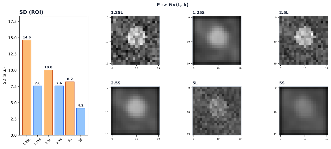
Schematic emulation, not a CT physics model. In filtered back-projection the kernel shapes the frequency response by filtering the projection data before back-projection; iterative methods implement the resolution–noise trade-off differently. Slice thickness relates to the slab sensitivity profile and averaging along z, producing partial-volume effects. No setting is universally best. The six labels correspond to the RIDER v3 settings; the images and numbers are synthetic and do not exhaust reconstruction parameter space.

For orientation, the schematic panel labels retain t, k, and SD, including 1.25L and 5S; these are illustration identifiers, not clinical values.

Slice thickness, spacing, and acquisition variables

Slice thickness and slice spacing are related but distinct. Thickness describes the slab represented by a slice and the associated averaging through that slab; spacing describes the distance between slice centres. They may have similar numbers in a routine stack, but they answer different questions about the image and its usable three-dimensional sampling. Both belong in the provenance of a quantitative analysis.

Dose and x-ray spectrum are acquisition variables, not alternate names for the six reconstruction settings. They can affect noise and the measured attenuation of materials, while contrast phase is a clinical-timing variable that changes the physiological context of an attenuation value. These variables may all change a measurement, but they do not become reconstruction replicates merely because they appear in the same examination. A study must record them and state which comparison treats them as fixed, varying, or out of scope.

The consequence for quantitative measurement

A useful working model is that a radiomic feature is a function of (image, mask, geometry, preprocessing). The image is itself a function of the acquisition and reconstruction choices, so the dependency can be written as feature = F(R(P; θ), mask, geometry, preprocessing). This is not a claim that a single variable explains every observed difference. It is a reminder that a feature value cannot be interpreted without the conditions that produced its image.

Fixed retained projection data P
(when re-reconstruction is supported)
    |
    +-- R(P; theta_A) --> image I_A
    |       |
    |       +--> F(I_A, mask_A, geometry_A,
    |                preprocessing_A) --> feature A
    |
    +-- R(P; theta_B) --> image I_B
            |
            +--> F(I_B, mask_B, geometry_B,
                     preprocessing_B) --> feature B

theta_A != theta_B, so feature A need not equal feature B.
A reconstruction-only contrast also requires the other feature inputs
to be controlled or explicitly modelled.

The figure makes this concrete: holding the synthetic source volume V_syn fixed in a schematic example does not force the six illustrative outputs J_theta or their simple ROI summaries to be equal. The values in the figure are synthetic and illustrate dependence on settings; they are not measurements from the RIDER collection.

Texture features often respond directly to changes in spatial frequency and noise. Shape features are computed from the mask and geometry, so a kernel may affect them indirectly when the mask is derived from the image or when the grid changes. The useful distinction is therefore conditional: do not assume texture is stable, and do not assume shape is independent without checking mask and geometry stability.

The practical rule is simple: record the reconstruction, report it with every result, and do not pool images from different reconstruction regimes unless that comparison is intentional and designed. A measurement that ignores this boundary cannot tell whether an observed difference belongs to anatomy, acquisition, reconstruction, or the later measurement procedure.

That boundary leads directly to the next modality. CT makes the role of reconstruction visible because transmitted x-ray projections are turned into an image under explicit choices. MRI begins from a different physical signal, and its image intensity and contrast must be understood through its own acquisition and reconstruction variables rather than by importing CT assumptions. The next chapter starts with that modality-dependent image-formation problem.

Sources

• Lee W. Goldman, “Principles of CT and CT Technology” — projection measurements, reconstruction, and CT-number foundations; transmission measurements, the logarithmic projection model, filtered back-projection, and Hounsfield units.
• DICOM PS3.3, CT Image Module, CT Reconstruction Macro, and Image Plane Module — the normative pixel, acquisition, and reconstruction metadata contract; normative CT values and reconstruction metadata; normative convolution-kernel, slice-thickness, and slice-spacing semantics.
• Binsheng Zhao et al., “Reproducibility of radiomics for deciphering tumor phenotype with imaging”, and Barbaros S. Erdal et al., “Are quantitative features of lung nodules reproducible at different CT acquisition and reconstruction parameters?” — reconstruction-dependent quantitative measurements; feature sensitivity to reconstruction settings; kernel/thickness effects and non-interchangeability of reconstruction regimes.
• Martin J. Willemink and Peter B. Noël, “The evolution of image reconstruction for CT—from filtered back projection to artificial intelligence” — filtered back-projection and iterative/model-based reconstruction.
• Tami D. DenOtter and Johanna Schubert, “Hounsfield Unit”, and Yousif A. Al-Naser and Dawood Tafti, “Computed Tomography Instrumentation and Physics” — HU orientation, protocol dependence, image noise, and partial-volume effects.
• Binsheng Zhao et al., RIDER Lung CT version 3, and Zhao et al., “Annotated test-retest dataset of lung cancer CT scan images reconstructed at multiple imaging parameters” — cohort, repeat-scan design, and six reconstruction settings.
• Binsheng Zhao et al., “Evaluating Variability in Tumor Measurements from Same-day Repeat CT Scans of Patients with Non–Small Cell Lung Cancer” — same-day repeat design and measurement variability.
• Abi Berger, “Magnetic resonance imaging” — the distinct magnetic/RF signal and pulse-sequence basis of the Chapter 2 transition.