Why image and mask resampling must differ

You resample a CT and its tumour mask to a common 1 mm grid. You use the same interpolator for both. The mask now contains voxel values of 0.4 and 0.7 — “40% tumour, 60% liver” — and shape and boundary features can silently change. This section is why image and mask resampling are deliberately asymmetric, what the interpolators actually do, why the HU clip comes after resampling in the TRACE-CT pipeline, and why that order is part of the measurement definition. The asymmetry is the key distinction; the operation order is the bridge into the measurement chapters that follow (Chapter 5).

Continuous values vs discrete labels

Resampling is unavoidable in radiomics (pipelines normalise to a common spacing) and in mask transfer — and the same operation must be done differently to the image and the mask, because of what the numbers mean.

The image holds a continuous quantity (HU, a roughly meaningful scalar field), so interpolating between neighbouring voxel values is legitimate: the true value at a point between two voxels is plausibly between their values.

The mask holds discrete labels. Interpolating “half tumour, half liver” between two label voxels yields a value that is neither label — meaningful only when a fractional representation is exactly what you intend. Some formats deliberately store per-voxel occupancy or probability values, and that is a valid representation; the mistake is letting a binary mask reach radiomics extraction as accidental fractional labels. So the two objects are normally resampled with different interpolators:

• Images: linear (or B-spline) interpolation — smooth, physically reasonable.
• Masks: nearest-neighbour — every output voxel takes the label of the nearest input voxel, preserving the existing discrete label set directly. This is also PyRadiomics’ own mask path.

Label-aware rule: nearest-neighbour keeps a discrete label set intact with no extra step. IBSI additionally permits linear (trilinear) mask interpolation followed by an explicit binarisation threshold — a valid alternative when that threshold is declared and pinned. What must not happen is a binary label map left fractional after interpolation: it breaks label integrity and can change boundary-dependent features.

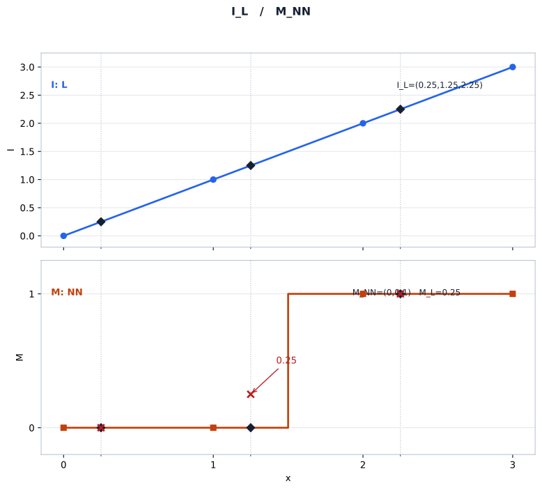
L denotes linear interpolation and NN nearest-neighbour label transfer. The fractional marker shows what must not be passed onward as a binary label; linear or trilinear mask interpolation is also valid when followed by an explicit declared and pinned re-binarisation threshold.

The interpolators, compared

Interpolator	Use for	Behaviour	Risk
Nearest-neighbour	mask / labels	every output voxel takes the label of the nearest input voxel; integer labels preserved	blocky boundary (expected)
Linear (trilinear)	image (safe default)	convex weighted combination of the 8 surrounding voxel values — stays within their range; fast, no overshoot	smoothing (degree is context-dependent)
B-spline	image (TRACE-CT’s frozen choice)	smooth piecewise-polynomial reconstruction	overshoot possible past the input range at sharp boundaries

The grid, precisely

A voxel grid is defined by the three quantities from the chapter’s opening section: origin (physical position of voxel [0,0,0]), spacing (physical step per voxel axis — the TRACE-CT RIDER case pairs series reconstructed at 1.25 mm and 5.0 mm slice thickness), and direction (the axis orientation in patient space). Resampling means evaluating the image on a new grid — different spacing, origin, or direction — and to compute each new voxel’s value you look at the input voxels around the corresponding physical location and combine them. The question is how you combine them — and the answer depends on what the numbers mean: continuous field or discrete labels.

Upsampling is not resolution

The TRACE-CT RIDER case pairs a 5 mm-thick reconstruction with a 1.25 mm-thick one of the same patient — two different reconstructions, not two samplings of one identical image. Put the 5 mm series on a 1 mm grid and you get roughly five times as many sample locations along z (the exact count depends on the imaged extent and the endpoint convention) — but no new anatomy. More samples ≠ more information. The 1 mm grid evaluates an interpolation of the 5 mm samples; it cannot recreate the high-frequency z detail the 5 mm reconstruction already lost during reconstruction itself (Chapter 1’s reconstruction case). Neither direction creates acquired resolution, and both can alter values: upsampling fills a finer grid with inferred values, which can smooth, overshoot, or otherwise differ from a native measurement; downsampling removes detail and can blur or alias. TRACE-CT’s resampling of the 1.25 mm series to a common 1 mm isotropic grid is a project decision about pipeline consistency — not a change that leaves every value untouched.

What B-spline actually does (and why it can overshoot)

• Nearest-neighbour copies the closest input voxel. Discontinuous, label-safe.
• Linear/trilinear computes a convex weighted combination of the eight surrounding voxel values — in 3D, the 8 corners of the surrounding cube, weights from trilinear interpolation. It can never leave their range: a convex combination of numbers is bounded by their min and max. How much it smooths depends on context — the sampling, the structures, and how many operations are chained.
• B-spline reconstructs the image as a smooth piecewise-polynomial model (a spline with compact support — each polynomial piece only “sees” a few voxels) and then evaluates that model at the new locations. It is tempting to picture the raw samples as the spline’s local control coefficients, but treat that as intuition only: implementations derive the polynomial coefficients from the samples, and details differ between libraries. The safe statement is that the output voxel is not an average of inputs; it is the value of a smooth piecewise-polynomial model built from them.

That is the whole intuition: linear answers “what is the weighted average here?”, B-spline answers “what does the smooth piecewise-polynomial model built from my neighbourhood say is here?”. And because a higher-order smooth interpolation is not constrained to stay within the local sample range, it can overshoot around sharp transitions — a boundary between air at −1000 HU and tissue at +100 HU can yield interpolated values below −1000 or above +100 (like a flexible ruler bending around a corner, the fitted curve can leave the range spanned by the two samples). That is overshoot: a property of higher-order smooth interpolation at sharp edges, not an error of the interpolator. Whether B-spline is the right choice is a design decision, not a law: it is TRACE-CT’s frozen image interpolator (chosen for smooth-region fidelity), and linear — or other — interpolators are also legitimately used elsewhere. What is scientifically required is to justify, freeze, and report the interpolator, because it is feature-determining — and when the choice is B-spline, to deal with the overshoot, which is exactly what clipping does (below).

Clipping, numerically

TRACE-CT clips HU to [-1000, +400] after resampling:

input HU      clipped HU
−1200    →    −1000     (below range: pinned to floor)
−850     →    −850      (inside range: unchanged)
 120     →     120      (inside range: unchanged)
 900     →     400      (above range: pinned to ceiling)

Clipping modifies image intensities, nothing else — the mask, the voxel count, and the geometry are untouched. Every voxel value below −1000 becomes −1000; every value above +400 becomes +400. Two effects in one operation: (1) it enforces prespecified analysis bounds, which can change the observed intensity distribution and its discretisation; (2) it fixes the intensity range the discretisation will see, which matters because binWidth-discretised texture features depend on that range (Chapter 6).

Clipping is not resegmentation. PyRadiomics has a separate setting, resegmentRange, that removes voxels from the mask whose intensities fall outside a range — it changes which voxels belong to the ROI. Clipping changes what values those voxels contribute. TRACE-CT clips image intensities externally and keeps resegmentRange at None (no mask change). Confusing the two silently changes both the intensity distribution and the ROI.

Operation order is part of the measurement definition

Is resample → clip the same as clip → resample? No — they are not algebraically equivalent, and a tiny thought experiment shows why. Take a one-dimensional boundary, input samples …, −1000, −1000, +350, +500, …:

• Clip first: +500 → +400; the samples are now …, −1000, −1000, +350, +400, …. Now interpolate at the midpoint between +350 and +400: linear gives +375; B-spline gives something smooth nearby. Clipping first changes the samples the interpolator sees — the pre-clip structure of values outside the range (was it +500 or +900?) is erased before interpolation ever sees it. It does not confine the output to [-1000, +400]: higher-order interpolation such as B-spline can still overshoot the range of its (already clipped) samples.
• Resample first: the interpolator sees the unclipped values (+350, +500) and produces its smooth estimate between and around them (+425 at the midpoint, possibly overshooting past +500); only then does the clip pin the final values into [-1000, +400] (+425 → +400).

Same input, same target grid, different measured intensities at the boundary — so a texture feature computed from them can differ too. Neither order is “wrong”; they are different measurement definitions. TRACE-CT froze:

DICOM pixels → HU (RescaleSlope/Intercept)
  → external 1 mm isotropic resampling (B-spline image, NN mask)
  → clip to [-1000, +400] HU
  → PyRadiomics

and froze it in that order for stated reasons: this is the committed implementation and configuration of the TRACE-CT pipeline, checked by regression tests at the pinned commit (the resample-then-clip order and configuration are part of what is checked). That validation establishes what the pipeline is — it is not a claim of clinical validity, optimality, or that a B-spline overshoot occurred in every series. What the order does guarantee is that clipping bounds the final sample values immediately before extraction. This is the frozen TRACE-CT measurement definition — not a claim that clip-after-resample is universally the only correct order. What is universal is the discipline: state the order, pin it, and do not change the prespecified primary pipeline after seeing outcomes without declaring a new analysis — a prospective method revision is legitimate, but it is a new measurement definition, not the same one, because changing the order changes the measured quantity (the anti-tuning guardrail, later recast as the measure-before-intervening case study in Chapter 6).

No double resampling

One more frozen rule that follows from the same logic. TRACE-CT resamples to 1 mm externally, before PyRadiomics is invoked. The PyRadiomics parameter file therefore must not set resampledPixelSpacing — if it did, PyRadiomics would resample the already-resampled image again, applying a second interpolation operator to the data. Two interpolation passes are not the same measurement as one: the extra stage changes the pipeline and may alter the samples, with behaviour that depends on the interpolator (nearest-neighbour does not smooth at all, and linear does not overshoot the way B-spline can). The rule is the frozen TRACE-CT design rule — external resampling or PyRadiomics resampling, never both — a project decision against an unintended duplicate stage, not a universal law that no pipeline may ever resample twice; TRACE-CT verifies it by loading the parameter file through the actual pinned extractor and checking that the effective resampledPixelSpacing is None (Chapter 5’s operational-definition section).

The asymmetric resample, in code

import SimpleITK as sitk
# image: B-spline; mask: nearest-neighbour — to the SAME reference geometry
resampled_img  = sitk.Resample(img,  ref_img, sitk.Transform(), sitk.sitkBSpline,
                               0.0, sitk.sitkInt16)
resampled_mask = sitk.Resample(mask, ref_img, sitk.Transform(), sitk.sitkNearestNeighbor,
                               0, sitk.sitkUInt8)

Note the deliberate asymmetry: same reference, same transform, different interpolator and background value for image vs mask. This is the SimpleITK bridge from the chapter’s opening section doing its job — it carries geometry with the image, so resampling is a geometric operation, not an array reshuffle.

Two “partial volumes”: acquisition physics vs digital resampling

The word partial volume is used for two different things, and separating them keeps the causal story honest.

Physical / acquisition–reconstruction partial volume. A reconstructed voxel or slice represents a finite spatial extent — a 5 mm-thick reconstruction has finite through-plane sensitivity on the order of its slice thickness, not the sensitivity of an infinitely thin plane. (The exact sensitivity profile depends on acquisition and reconstruction; it is not necessarily a uniform average over a 5 mm box.) Tissue within that sensitivity profile contributes to the reconstructed value, so thick slices mix structures and lose spatial detail. Crucially, this happens inside the scanner/reconstruction: by the time a digital image exists, this information is already gone. No later resampling — in either direction — can recover it.

Digital resampling / downsampling. This operates on an already reconstructed digital image: interpolation estimates values on a different grid. Downsampling to a coarser grid can remove detail, smooth, alias, or blur boundaries — the exact behaviour depends on the interpolator (nearest-neighbour does not average anything; it picks a source voxel; B-spline/linear compute smooth estimates). This is a mathematical operation on samples, not a re-measurement of a tissue mixture.

anatomy
  → scanner acquisition + reconstruction (physical partial volume: finite
    voxel/slice support; thick reconstructions mix structures — loss happens HERE)
  → reconstructed voxel values (the digital image)
  → later digital interpolation / resampling (grid change; interpolator-dependent)

The ordering matters because it assigns the irreversible loss to the right stage: resampling a 5 mm series onto a 1 mm grid cannot undo the through-plane detail the 5 mm reconstruction already lost — it only re-evaluates the surviving samples on a finer grid (see upsampling is not resolution, above). What digital downsampling adds is its own, interpolator-dependent change to boundary sharpness and texture — at a tumour boundary a coarser grid makes the boundary representation blurrier or blockier, which changes volumes, edge sharpness, and texture features. That downstream effect is expected behaviour of the pipeline, not a bug — but it is why every radiomics analysis that involves resampling must report, as applicable, the target grid (size, origin, spacing, direction), the transform, the interpolator, the applicable defaults, and the operation order — or the feature is irreproducible.

The chapter’s punchline

Everything in this chapter converges here:

A radiomic value is a function of the image samples, the ROI representation, the complete geometry, the preprocessing, and the feature implementation. Interpolation and discretisation are preprocessing choices, not parts of geometry. Change any of these and the measurement definition changes — and the feature value can change, even though the underlying anatomy did not.

A short variant sharpens the point. Resample both image and mask to 2 mm isotropic (from 1 mm) using nearest-neighbour for the mask and B-spline for the image, then recompute a texture feature: the value changes. The new value is not “wrong” — it is the feature under a different geometry, which is a legitimately different quantity. The error would be to report the new value without recording the new spacing and interpolator, or to compare it to a value computed at 1 mm as if they were the same measurement. A resampling change can alter feature values, and it always changes the measurement definition even where a value happens to come out the same; the discipline is to pin and report the target geometry so that any comparison is between like and like. A feature “changed by resampling” is only a problem if you did not notice you changed the pipeline.

This is why IBSI fixes a processing workflow, why PyRadiomics lets you pin resampling parameters, and why TRACE-CT commits a parameter file (configs/pyradiomics_params.yaml) with fixed binWidth and spacing rather than leaving them to defaults. The feature is not a property of the tumour; it is a property of the tumour under a stated pipeline. The chapters that follow exist to make that statement precise.

The last step of the chapter is to stop reading and look: the case study turns every concept above into something you can verify with your eyes.

Sources

• Zwanenburg A, Vallières M, Abdalah MA, et al. The Image Biomarker Standardisation Initiative: standardized quantitative radiomics for high-throughput image-based phenotyping. Radiology. 2020;295(2):328-338. PMID 32154773. doi:10.1148/radiol.2020191145. (PubMed; published full text: PMC7193906) — IBSI reference: interpolation algorithms and partial-volume effects in the ROI mask.
• PyRadiomics documentation — Customizing the extract: resampledPixelSpacing, interpolator, resegmentRange, and parameter files. (pyradiomics.readthedocs.io/en/latest/customization.html)
• SimpleITK documentation — Fundamental Concepts: Resampling, and the ResampleImageFilter API reference. (simpleitk.readthedocs.io/en/master/fundamentalConcepts.html#resampling)
• DICOM PS3.3, CT Image Module — Rescale Slope (0028,1053) and Rescale Intercept (0028,1052), with the output-units equation. (dicom.nema.org/medical/dicom/current/output/chtml/part03/sect_C.8.2.html)
• Zhao B, Schwartz LH, Kris MG, Riely GJ. Coffee-break lung CT collection with scan images reconstructed at multiple imaging parameters (Version 3) [Dataset]. The Cancer Imaging Archive. doi:10.7937/K9/TCIA.2015.U1X8A5NR. (doi.org/10.7937/K9/TCIA.2015.U1X8A5NR) — public RIDER collection identity and licence; the 1.25 mm and 5.0 mm slice-thickness labels used in this section are the TRACE-CT project’s targets, not general dataset settings.
• TRACE-CT radiomics pipeline (bounded case evidence) — frozen preprocessing implementation, parameter file (configs/pyradiomics_params.yaml), and drift tests at commit 7aaf308c76ed2718fd0b364d1cde856969711b72. (commit 7aaf308)